Anova

Fungsi Anova

Menguji perbedaan variasi antar kelompok (lebih dari 2) variabel yang akan kita uji
Kita akan menguji household income and happiness
Research Question: apakah terdapat perbedaan tingkat kebahagiaan ditinjau dari tingkat pendapatan?

Library

library(psych)
library(tidyverse)
library(rstatix)
library(report)
library(here)

Membaca data

data pengukuran tingkat kebahagiaan
tingkat DIY

income <- read_csv(here("datasets", "income_happiness_diy.csv"))
str(income)

spc_tbl_ [913 × 4] (S3: spec_tbl_df/tbl_df/tbl/data.frame)
 $ Provinsi  : chr [1:913] "Di Yogyakarta" "Di Yogyakarta" "Di Yogyakarta" "Di Yogyakarta" ...
 $ Income_ind: num [1:913] 5 5 5 NA 5 4 1 3 4 5 ...
 $ Income_hh : num [1:913] 5 5 5 5 3 4 2 1 1 1 ...
 $ Happiness : num [1:913] 6 8 7 6 6 6 9 8 5 8 ...
 - attr(*, "spec")=
  .. cols(
  ..   Provinsi = col_character(),
  ..   Income_ind = col_double(),
  ..   Income_hh = col_double(),
  ..   Happiness = col_double()
  .. )
 - attr(*, "problems")=<externalptr>

Visualisasi awal

income |> ggplot(aes(Income_hh, Happiness, color = Income_hh)) +
  geom_jitter()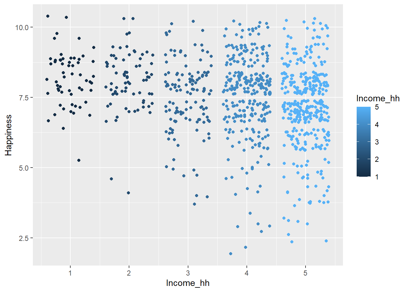

Membuat boxplot

income |> mutate(income_fct = as.factor(Income_hh)) |> ggplot(aes(income_fct, Happiness, color=Income_hh)) + 
  geom_boxplot()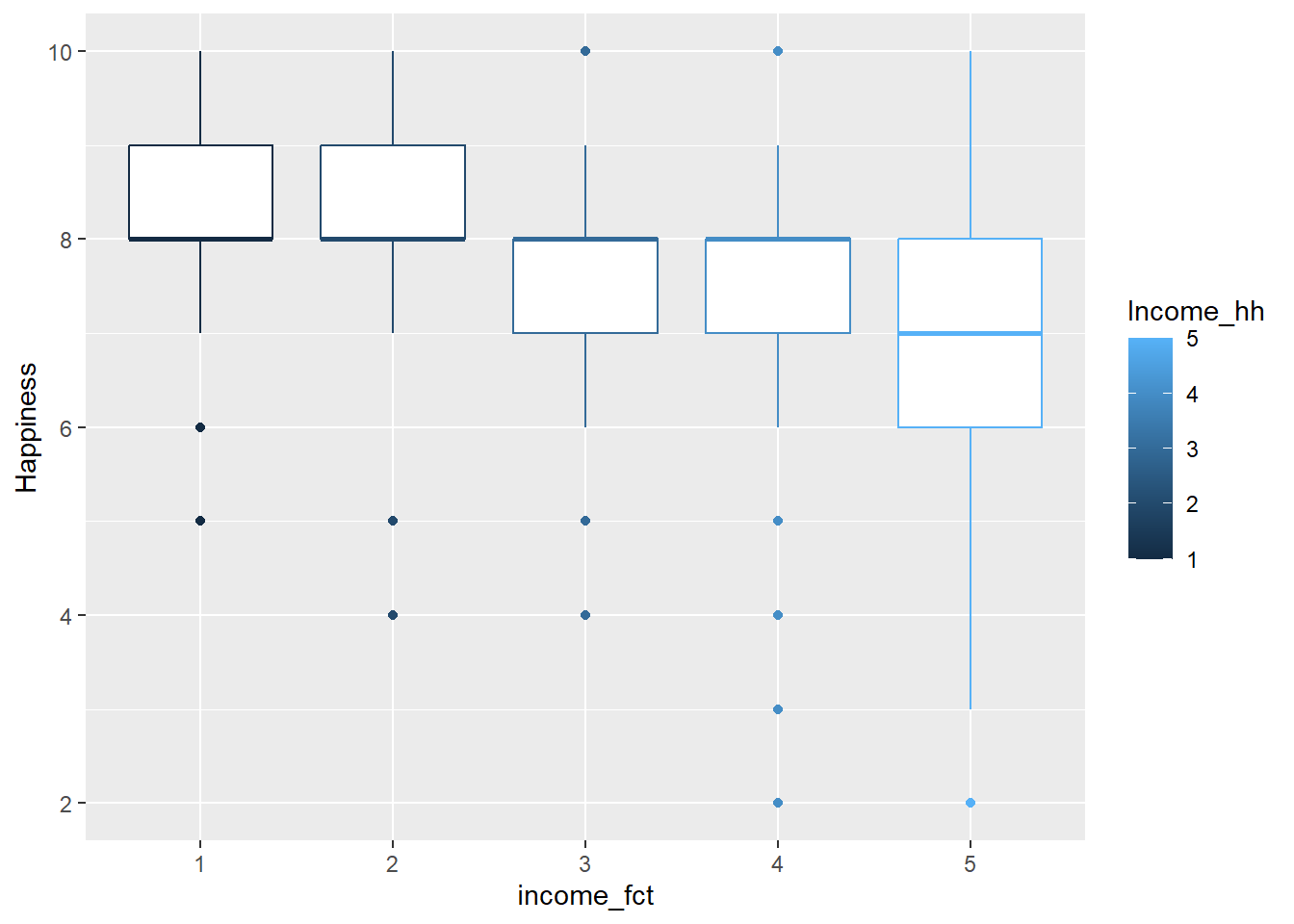

Deskriptif

income |>
  group_by(Income_hh) |>
  get_summary_stats(Happiness, type = "mean_sd")

# A tibble: 5 × 5
  Income_hh variable      n  mean    sd
      <dbl> <fct>     <dbl> <dbl> <dbl>
1         1 Happiness    58  8.22  1.03
2         2 Happiness    73  8.10  1.03
3         3 Happiness   123  7.50  1.26
4         4 Happiness   288  7.58  1.46
5         5 Happiness   371  7.17  1.46

Uji anova

beda <- aov(Happiness~Income_hh, data=income)
summary(beda)

             Df Sum Sq Mean Sq F value   Pr(>F)    
Income_hh     1   87.2   87.24   45.71 2.45e-11 ***
Residuals   911 1738.8    1.91                     
---
Signif. codes:  0 '***' 0.001 '**' 0.01 '*' 0.05 '.' 0.1 ' ' 1

Effect Size

A small effect size is about .01.
A medium effect size is about .06.
A large effect size is about .14.

report(beda)

The ANOVA (formula: Happiness ~ Income_hh) suggests that:

  - The main effect of Income_hh is statistically significant and small (F(1,
911) = 45.71, p < .001; Eta2 = 0.05, 95% CI [0.03, 1.00])

Effect sizes were labelled following Field's (2013) recommendations.